Category: Projects

This project was done for a Bachelor project together with colleagues Juraj Peršić, Lucija Kopić, Niko Višnjić, Tin Serdar, Borna Vukadinović, Marsela Polić and  Goran Popović.

Here is a copy of Goran’s post about this project.

—————————————————————————————————————————————-

Project had mythological background: Hercules (quadcopter) needs to group a herd of cattle (mobile robots) in the stable (black square).

Quadrotor

Parrot AR.DRONE 2.0 has a camera which records the ground beneath it. Camera is used for a localization of the quadcopter and to find a stable and the mobile robots. Quadcopter was communicating with the notebook which processed recorded video and controlled the position of the quadcopter.

At the beginning the quadcopter searched for the platforms and the stable. When they were found, quadcopter had to calculate which platform was most likely to escape from the arena and direct that platform to the stable.

Mobile platforms

mOway robots were used to simulate the cattle. Each platform had an IR proximity sensor and a colored triangle on top. Platforms were moving forward and then rotated around themselves. The distance and angle which defined the trajectory were randomly selected every time. After stepping in the stable, platform would stop and stayed there.

When the IR proximity sensor had sensed that the quadcopter is above it at height smaller than set, platform stopped moving and started rotating until the quadcopter moved.

Image processing

OpenCV library was used in image processing. Every second an image from the video was processed in order to find the location of the quadcopter, platforms and stable. The arena was split in 9 squares with gray stripes of different width so that the crossings could help in localization of the quadrotor. Furthermore, mobile platforms had colored triangle which enables differentiate platforms and determine their orientation.

 

 

 

 

 

 

— written by Goran Popović

—————————————————————————————————————————————–

More about the project can be read here Project_presentation_cro  but unfortunately it is in Croatian.

This project was done for the “Elektroboj” competition together with colleague Goran Popović.

Here is a copy of his post about this project.

—————————————————————————————————————————————–

The goal of this project was to construct a 3D printer which moves in XY plane with DC motors instead usually used stepper motors. The idea was that continuous DC motors with encoders for feedback information will be faster and will produce better look of the printed part. When stepper motors are used, there is no feedback information about the position of the printing head. That is not a problem in most cases since the forces in XY plane can’t produce such momentum on the axis of the stepper motor to cause a slip in motor’s steps. If one would want to print faster, inertial force of the massive printing head could cause slippage which would result in unusable printed part.

Electronics

An open-source solution uses RAMPS shield with Arduino Mega microcontroller board. The existing solution was adapted so that the output signals from RAMPS board were forwarded to the board with 2 H-bridge chips and 2 Arduino Pro Mini microcontroller boards. Arduino Pro Mini converts signals for stepper driver (DIR- direction & STEP) into PWM signal which controls DC motors over H-bridges.

Image shows RAMPS board with a newly designed PCB for 2 Arduino Pro Mini and H-bridges.

Beside 2 DC motors that control X and Y axis, there are also 3 stepper motors, two for Z axis and one for filament extrusion. Each axis had two end stoppers that limited the working area of printing head.

Software

Software was divided in three parts: Solidworks for the design of 3D models, Cura for converting a STL model in G-code (machine language) and Repetier as G-code interpreter.

Since some parts needed a modification, new modified parts were designed in Solidworks, and were printed on the 3D printer. In order connect command chain between STL model and head of the printer, Cura and Repetier were used. Cura slices the STL model in small steps that the model consists of. G-code command is given to each of these steps. Repetier reads the G-code and sends signals to RAMPS board that then controls the motors.

Arduino Pro Mini that were uses to control DC motors were running PID regulator program. Signals DIR and STEP from the RAMPS board were used to change a position reference of the DC motors. The reference was then compared to the value received from the encoder.

Mechanical construction

It was decided to use Prusa i3 model as a base and adapt it to the model with DC motors.

Except wooden frame which was cut on CNC machine and 2 downloaded STL parts, everything else was designed by ourselves.

Images show printing plate which moves in Y axis.

DC motor for X-axis which moves printing head.

Summary

In this project 3D printer with DC motors was constructed and it could precisely position in the all three directions and melt the filament through the printing head. The remained problem was that the melted filament wouldn’t stick to the printing plate. Due to the project deadlines we did not find the solution for that problem.

— written by Goran Popović

—————————————————————————————————————————————-

More about the project can be found in documentation  Project_documentation_cro and  presentation Project_presentation_cro, but unfortunately both of them are in Croatian.

Science and technology are today moving in the direction of automation and autonomy of the systems. Detection of vegetation along the roads is one of a series of ideas that seeks to achieve the autonomy of the vehicles in traffic without the presence of the driver. By analyzing the images of captured environment it is necessary to determine which parts of the image are vegetation, and which are not. Due to the complexity of the problem, deep convolutional neural network which is trained on a large number of examples is used. After that, the goal was to examine the quality of the network on several images that were obtained as a result of the network. In this way it was possible to create a visual impression of the quality of the network.

Introduction

The environment around the vehicle is recorded with the camera. We wanted to be able to determine what parts of the image are vegetation and what is not. This task cannot be achieved only by image analysis because there are too many variations that cannot be formally described. From this reason we moved in the direction of neural networks which are able to recognize patterns on the basis of a large number of examples. In this case, due to the complexity of the task, number of samples is very large (about 500,000). Therefore deep convolution neural network were necessary so that treatment could be in a finite amount of time. Training and testing was performed on GPU in order to reduce processing time needed.

The complexity of the problem lies in the fact that vegetation does not always mean only “green grass”. A large number of variations are possible; eg. different seasons which change vegetation color, the presence of leaves in autumn, shadows, bark of trees, colorful flowers, etc. Also along the curb are often parked cars or the camera captures the people passing by. For this reason, the color is not good enough criterion for identifying the vegetation.

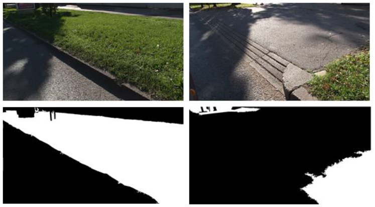
For training the network a large number of images of lots of different situations is needed. For each image manually tagged masks are needed. Masks are the desired output of the network, or one-dimensional black and white image in which the vegetation is designated with1, and the rest is 0. Examples of images and a corresponding mask are shown in figures below.

Deep convolution network

Deep networks are networks with many hidden layers between the input and the output layer. Specifically in this case, we used  deep convolution neural networks that operate on the convolution and image compression. The importance of these networks is great as it helps to extract key features to classify each individual pixel.

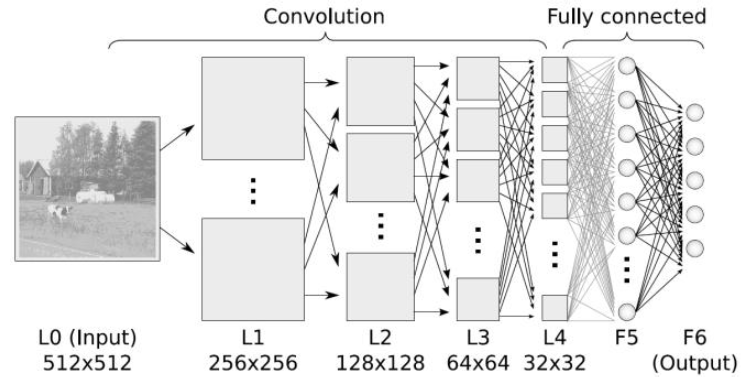
Figure above shows a typical structure of a deep neural network. The entrance can be one monochromatic images or multi-channel color image. Then alternating array of convolutional and pooling (compression) layers follows. At the end are several fully connected layers (classical perceptron) which are two-dimensional (including the output layer). Typical deep convolutional network has around ten layers. Convolution layers and pooling layers have two-dimensional “neurons” that are often called “feature maps” and which in each layer are becoming smaller. The convolutional layers are connected to the previous layers, and adjust connection weights by learning. The pooling layers do not learn any weights.

These networks are easier to be trained than other deep learning methods, and it is also possible to find more features, which can be passed through filters (which are practically layers of deep convolutional neural network). They also require relatively little preprocessing. In some cases, they were shown to work better than a man. But often they are criticized because of poor understanding of what is actually happening inside the hidden layers.

“Caffe” tool

We used the “Cafe” tool. It is a tool that runs the training of deep neural networks instead of us. In order to use “Caffe” tool, we had to adjust the input data in the appropriate format (LMDB). Then the network had to be designed; layers should have been named and sizes and interconnections defined (in .prototxt format). Location of test and validation sets of images had to be linked.

Parameters of training (solver.prototxt) had to be defined. Parameters include: the maximum number of iterations, after how many iterations validation follows, what is the rate of learning, etc. After the training, the network had to be tested.

Preprocessing of images

Two hundred pictures of different scenes were used as a set for training. But first few preprocessing steps were needed in order to obtain the final dataset for training. The image dimensions were 1080×1920 px which is too high and were reduced in both dimensions to the dimensions of 270×480 px.

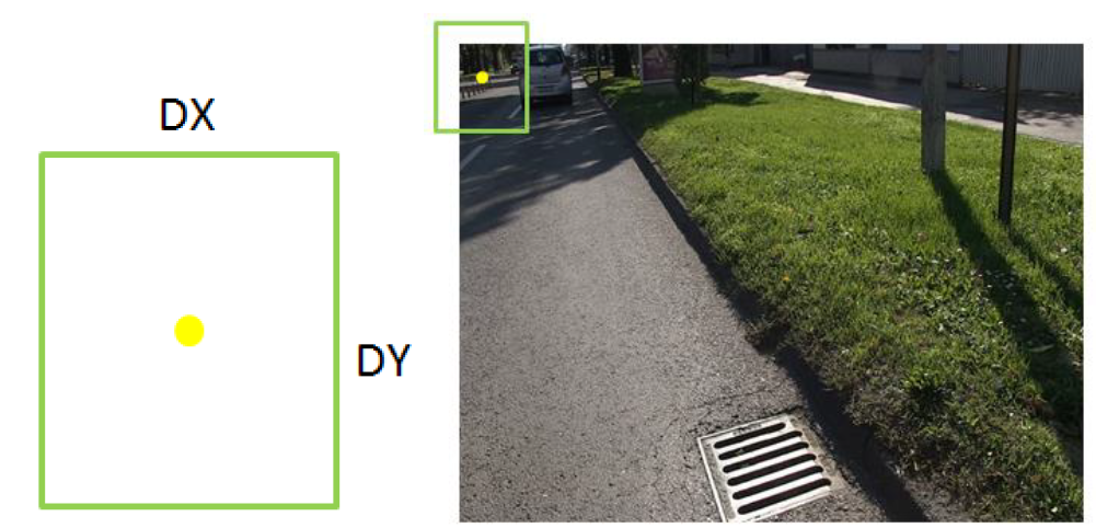
The input to the network is not the whole picture but a cutout frame of DXxDY pixels around the central [cx, cy] pixel. Using DXx DY surrounding pixel networks should conclude whether the central pixel is vegetation or not: there are two possible exits, 1 or 0. For each frame correct answer is also needed in order to train. The correct answer is value of [cx, cy] pixel in the mask image.

In order to improve training, large number of  DxxDY frames were cut out from each image and together with correct answer  stored in a file in the form:

crops_train / 3_1.jpeg 0
crops_train / 3_2.jpeg 1
…

This format is called LMDB. It is important that the test data consists of approximately the same number of positive and negative examples, and that they are uniformly spaced.

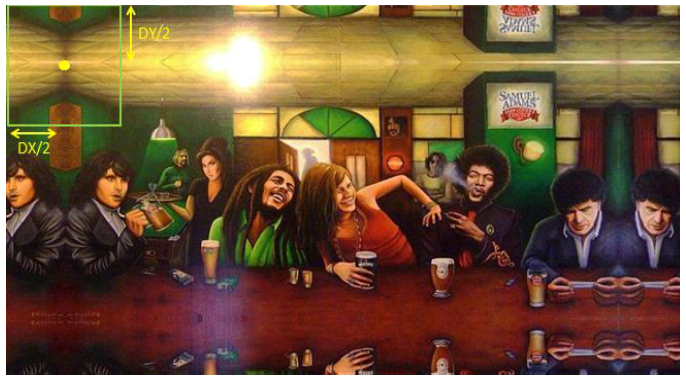
Since the boundary pixels also have to be classified it is necessary to expand the image around them so that there is also DXxDY pixel frame around them. Expanding is done by mirroring: on all edges of the image boundary DX/2 or DY/2 pixels is flipped and the images are stored. Only after this process is done, cutting the frames and converting to the LMDB format is done. All of this is shown in images below.

Since most of the networks are designed for the input data in the range [0,1], and the color values of pixels in the image are in the range [0,255] it was necessary to scale the value of all pixels.

Matlab script was written which performs all preprocessing that was mentioned so far:

– reduces images
– mirrors edges
– scales values to [0,1]
– cuts out frames at random coordinates
– saves frames as a separate files
– gives the names to the frames and stores the result in the LMDB file

Postprocessing and testing

Testing the quality of training networks was done on several images from the test set. Matlab script was written which takes one by one  image from the test set, reduces it to 270×480 px, scales values to [0,1], extends in the same manner as in the preprocessing, and then for each pixel cuts out a frame and sends into a neural network.

Network gives as a result two numbers; the probability that this pixel is 1 (vegetation), and the probability that the score is 0 (Others). After the results of the network, it is necessary to determine the threshold above which the percentage will determine whether it is vegetation or is not. Determination of percentages is done using ROC curves.

When threshold is defined, it is finally decided whether the network said 0 or 1 for each pixel. After that the resulting image is constructed. Visually it is possible to compare the resulting image and corresponding mask which represents the exact solution.

To determine the numerical accuracy of the network, this process is repeated for several pictures and in each image it is calculated as the number of exactly classified pixel values. Accuracy is calculated for each image, and finally evaluated to get the average accuracy of all images. All this is recorded in the .txt file.

Results

In trying to evaluate the work of each of proven neural network using MATLAB wrappers for Cafe for every given input (cut out the frame around [cx, cy] pixel images for testing), we got the same output from the network. We tried to solve this problem on different ways which included the review of everything done so far.

First we changed the architecture of the network several times, but each time the problem remained present. Then we tried the scaling of the input data to the interval [0,1]. Then we noticed that other people(from the Internet) reported the same problem , and we tried to apply the advice which they suggested, and that was the reduction of learning and mixing together for training, but even that did not help.

The last attempt was balancing the training set in a way that has exactly 50% of the positive examples for learning. Previously training set was created by randomly cutting out the frames from the images, ignoring their label, so the                 result was a significantly higher number of negative training examples. Training of these data with a rate of 0.0001 teachings caused the loss function through iteration learning slightly oscillates around the value of 0.70 from which we assumed that that was a local minimum from which with such a low rate of learning, function loss could not move. However, increasing the learning rate to 0.1 and then after training, network function loss slightly decreased, but still oscillated.

Conclusion

We examined the deep convolutional neural networks and designed several of them in an attempt to resolve the problem of detection of vegetation along the roads.

Matlab scripts for pre- and post-image processing were constructed. Preprocessing performed certain operations on the input images and created a data set for training and validation. Post processing takes the entire image and part by part (frame by frame) receives the result of the network. The goal is that these results match as good as possible with the corresponding mask, and thus except from the numerical accuracy of the network and visual the quality of a network.

Unfortunately, the final structure of the network that successfully detects vegetation has not yet been found. There were problems that the loss function during training network does not fall continuously but oscillate. Also after the end of training, when the testing is performed, it returns almost the same value for each input frame, and gives the same result regardless of the input.

Work on the problem will continue.

Acknowledgement

This project was a project on a Neural networks course and was done in a group of three students: Toni Antunović, Mladen Kukulić and me. The final report can be seen here (in Croatian unfortunately):   Project-text and the presentation (in English) here: Project-presentation.

Literature

• „Raspoznavanje objekata dubokim neuronskim mrežama“, Vedran Vukotić, Diplomski rad, FER 2014
• „Caffe: Convolutional Architecture for Fast Feature Embedding“, Yangqing Jia_, E. Shelhamer, Donahue, S. Karayev, UC Berkley
• http://caffe.berkeleyvision.org/ (access 20.12.2014.)

Introduction

Recognition of a person on the basis of retinal image is biometric procedure which uses the blood vessels pattern in the retina for recognition. Although it is not as popular as other identification procedures such as finger print, voice recognition, DNA analysis or iris or face recognition, retinal images recognition has some advantages over other techniques.

For example, when compared to finger print recognition it is more robust and precise. Fingerprint recognition is more sensitive to different finger position, scars and filths. When compared to voice recognition there is no problem of background noise and retina is less sensitive to changes due to illnesses or state of person’s health and mood. DNA analysis has huge disadvantage over most of other techniques; long processing time.

Drawbacks of retinal image recognition are somewhat uncomfortable process of taking picture, expensive equipment and potential changes of retina due to illnesses and astigmatism. This recognition technique is still not widely used. Most often it is used for gaining access to complexes with very high level of security. It is used by some of governmental agencies in USA, such as FBI, CIA and NASA.

Theoretical background

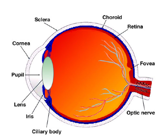
Figure above shows an eye with the marked most important parts. The figure shows that the retina is the inner membrane and is placed in the back of the eye. When the eye is focused, the light is projected on the retina. Due to the complex structure of capillaries that supply the retina with blood, the retina of every person is unique. The network of capillaries in the retina is not genetically determined so that even in identical twins this network is not similar. Although blood vessels in the retina can be changed as a result of diabetes, glaucoma or retinal disorders, retina remains unchanged from birth to death. For these reasons, the identification by the image of the retina is one of the most accurate biometric identification methods. The inaccuracy of this method is one of 10 million.

Image of the retina is obtained by a scanner which emits an infrared beam of low energy in the eye of the person looking into the eyepiece scanner. Beam moves over the retina by a standardized way. The capillaries in the retina absorb more light than tissue that surrounds them so that reflection during scanning varies. After that, the images are digitized and processed.

The algorithm that is used is divided into three steps. In the first step, the method of amplitude segmentation determines the center of optical disk. In the second step, the modified filter produces binary image in which vessels are expressed. In third step, the two binary images of the retinas are aligned by the centers obtained in the second step and then their difference is determined and, based on result it is decided whether the two images are from the same person.

Algorithm

The first task of the embodiment consists of finding of position of an optical disc. Optical disk area is the brightest part of the image and therefore its location can be determined by the amplitude image segmentation. This position is required later for the alignment of images in order to make their comparison.

First we need to blur the image by convolution with averaging filter. Then the extraction of middle part of the picture is done. This step is required because of the possible appearance of bright parts on the edges of the image that could affect the accuracy of the solution. It is extracted by multiplying the elements of the original image with a mask consisting of the units in the center and a zero at the edges. Since the optical disc is on all images located near the middle of the picture, removal of the peripheral areas does not lead to the loss of the accuracy of detection.

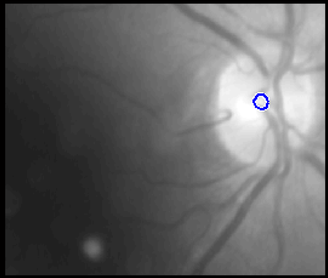
Following the removal of unnecessary parts, the brightest part of the picture has to be found. The first step in this procedure is the preparation of the histogram and the percentages of the light part. It was experimentally obtained that for most cases the best results are obtained when it is assumed that the proportion of bright areas is approximately 1.5% of the total area of the histogram. Then binary mask is calculated using the boundary calculated from the histogram. The last step is to calculate the coordinates of boundaries of optical disc from these masks. The result of detection of the optical disk is shown in figure below.

The second task is the detection of vessels using the matched filter. In contrast to the detection of the edges, the matched filter takes into account the shape of the object to be detected and gives results with much less discontinuity. When designing matched filter four characteristics of blood vessels in retinal images were observed:

1. Blood vessel have a small curvature and can be approximated with array of linear segments
2. Since they reflect light less than other parts of the retina, they look darker than the background. The vessels almost never have sharp edges. Although the intensities of the various vessels vary, they can be approximated by a Gaussian curve.
3. Although the width of the vessels decreases as the vessel moves away from the optical disc, such a change is gradual.
4. It can be assumed that the vessels are symmetrical in length.

Matched filter should have the form of an object that we want to detect. Taking into account the above listed characteristics of vessels, matched filter had a form:

where d is the width of blood vessels, and σ determines the width of Gaussian curve.

In two-dimensional space it is necessary to consider that the vessels may occur at any angle and that the filter has to be rotated to all possible angles (0-180). In theory Gaussian curve is of infinite length so here it is determined that will be cut to ±3σ. Length of vessel segments that we want to detect is indicated by L. Thus, the size of the mask that defines a custom filter is L*6σ. The formula for calculating the coefficients of the masks is:

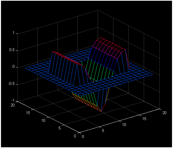
Following already said, mask has the following form: L same lines where the line is limited by Gaussian function. In our case we selected L = 9 and σ=2. For the default parameters mask is shown in the picture below.

After generating the mask it needs to set its mean value to 0. This is done so that the mean value is calculated by the formula

and thereafter from each coefficient subtracting this mean value. Then the mask is normalized by dividing with the maximum coefficient in the mask.

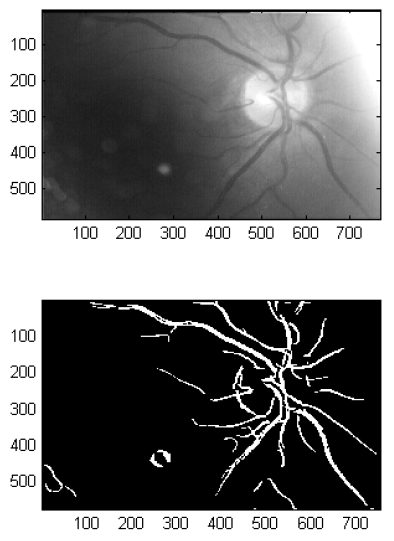
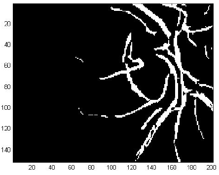
So that the coefficients of the mask would not be lost in the rotation, the mask is extended on each side with zeros. This allows usage of a mask of the same size for every angle of filtration. First, the mask is rotated for a certain angle and then the convolution is performed. The binary image is obtained by choosing the threshold value from convolution result. The threshold is determined automatically so that 4% points with maximum values after filtration are declared as vessels. Increment step of angle in this case was 10 degrees. After rotation for all angles, the images are combined using the OR operation into a single image. At the end of the binary image, objects that are smaller than 125 pixels are removed, in order to remove slightly detected blood vessel and other unimportant objects. The result of detection of vessels with mentioned algorithm is shown in figure below.

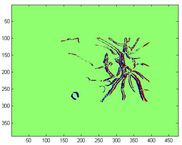
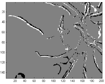
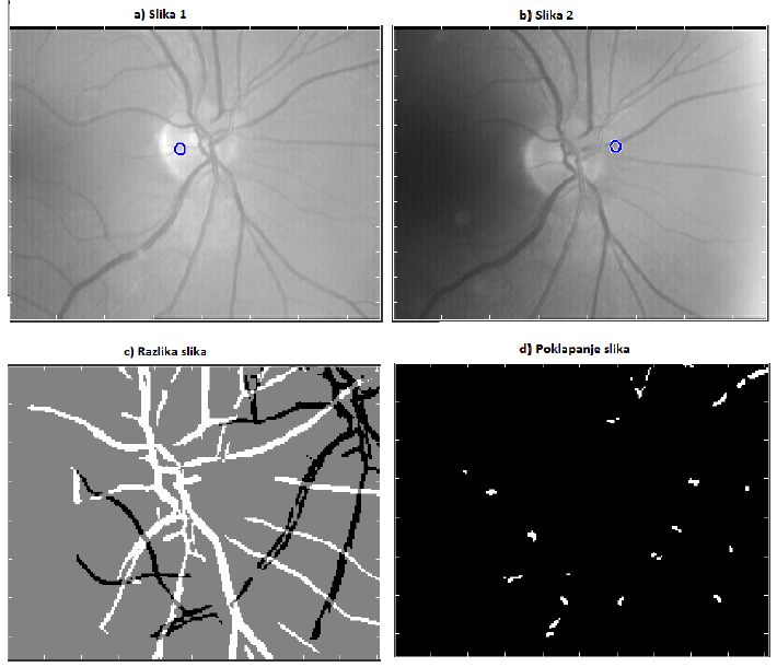
Decision whether to two different images of the retina belong to the same person shall be based on the difference of previously calculated binary image. The problem in the process of subtraction is fact that the images are often translated and rotated for a smaller angle. To solve this problem it is necessay first to set a reference point in the pictures. The selected reference point is the center of the optical disk obtained by amplitude segmentation and it serves to align the image in the process of subtraction. The difference image is calculated by subtracting two binary images. The process of subtraction begins by subsampling the images for a factor 2 in order to reduce the calculation time. After that it is necessary to expand the image and overlap them. As seen in figure below, overlapping the original images usually gives some major deviations. To achieve the best possible overlap, one image is taken as a reference, and the other is translated to positive and negative horizontal and vertical direction by 25 pixels with the steps of 1 pixel and rotated from -5 to +5 degrees in steps of 0.5 degrees. After each transformation the difference of two images is computed and result is stored in order to find the smallest value.

After the series of rotations and shifts the smallest difference is obtained, and now it is needed to decide on whether the images of the retina belong to the same person. This process begins with the rotation and translation of one image with the obtained parameters for which the smallest difference was calculated. After that one binary image is multiplied by a factor of two, and the second binary image is subtracted from it. In the newly created image the pixels with value 1 represent the overlapping vessels. The measure for the final decision is a percentage of overlapping pixels in the new image. Example of two image differences is visible and calculation of overlapping is shown in figures below.

.                      

Results

For most images algorithm gives good results. For pictures of the same person retina which are slightly different algorithm gives the percentage of pixels aligned above 90%. For pictures of the same person retina which are very different, for example, different contrast and brightness or a large difference between the centers of the optic nerves, percentage of alignment is between 60% and 70%. For images of different people’s retinas, aligned percentage is between 20% and 30%.

The inability to recognize can occur when on one of the image optical disc is not well recognized. An example of this case is shown in figure below. In figure optical drive is not properly recognized and is far from the true origins of the nerve. Erroneous determination of the optical disk comes mostly with images that are brighter than the average brightness of all images of the retina in the database. Then the selected value of 1.5% for determining the optical disc is not sufficient and false detection occurs.

Conclusion

Recognition of a person based on the image of the retina is a technique that is not very extensive, but has a number of advantages over the procedures for identification which are currently widely used. Retina is unique to each person and is very resistant to change. Moreover, a network of vessels in the retina is very complex. These properties make the image of the retina interesting for an application of identifying persons.

Given that the two images of the same retina are not completely identical, and that is possible to have a small translation or rotation when capturing an image, it is necessary to determine an element in the image as a reference. The ideal showed an optical disc. The area in most cases is the brightest area in the image. In addition, in this part, the network of vessels is the densest and most complex, so it is enough to make comparisons between image area located in its immediate vicinity.

In order to prevent the influence of the brightness of image on the results it is necessary to detect only parts relevant for comparison; that is network of vessels. Detection of vessels was performed using matched filter because it takes into account the shape of the object that we want to detect and gives results with much less discontinuity. Once we have extracted all the necessary data, the comparison of two images from databases followed. When comparing, one image is taken as a reference, while the other is translated and rotated. When the best fit is found the percentage of overlapping pixels from the original image is calculated. On the basis of this number it is concluded whether the images belong to the same person.

Acknowledgement

This project was a project on a Digital Image Processing and Analysis course and was done in a group of four students: Antonio Benc, Ante Gojsalić, Lucija Jurić and me. The final report can be seen here (in Croatian unfortunately):  Project_report and the presentation (in English) here:   Project_presentation

Literature

[1] C. Marino, M. G. Penedo, M. Penas, M. J. Carreira F. Gonzales, “Personal authentication using digital retinal images”, Springer-Verlag London Limited, January 2006

[2] S. Chaudhuri, S. Chatterjee, N. Katz M. Nelson, M. Goldbaum, “Detection of Blood Vessels in Retinal Images Using Two-Dimensonal Matched Filters”, IEEE Transactions on Medical Imaging, vol. 8, no. 3, September in 1989.

Project description

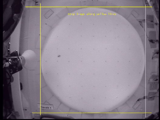
The goal of the project was to develop and analyze the model of bee movement in a field of CASUs (Combined actuator sensor units), which could be later used as a part of EU project ASSISIbf („Animal and robot Societies Self-organize and Integrate by Social Interaction (bees and fish)”). ASSISIbf is project whose goal is to create robots that are able to develop communication channels to animal societies (bees and fish) on its own, which would later be used to lay new foundations on the way how humans can interfere with animal societies in order to manage the environment. The animals used in ASSISSIbf project are shown on images below.

Bees like heat, light and vibrations. In this project bee’s reaction and movement in a field with a temperature gradient was researched. Two models were proposed: one in which is assumed that the bee can feel and detect temperature gradient (possibly with tentacles) and another one in which is assumed that bee can detect temperature and also has a memory to log position and belonging temperature.

Data about bee’s real movement were acquired from video materials made on experimental setup. Image of real arena where 1 to 3  days old bees were recorded is shown in figure below. This “biological” part of project is done at TU Graz.

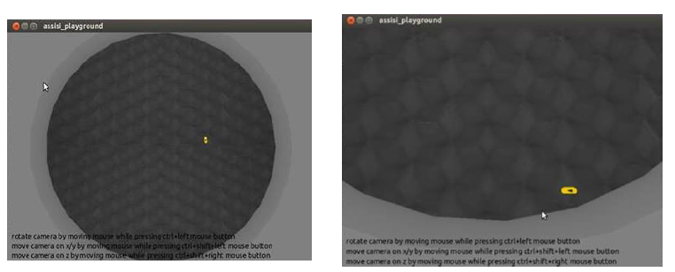
Moves were analyzed and compared with proposed models. In Enki simulator (image below) a control system for bees was implemented to visualize movement but also to enable future simulation of the whole system of bees and CASU units.

More details  will be published soon.

Acknowledgement

This project was my Bachelor thesis project under the mentorship of Professor Stjepan Bogdan. The full text of bachelor thesis can be downloaded here (in Croatian unfortunately):   Bachelor_thesis-text and the presentation from the thesis defense can be seen here: Bachelor_thesis-presentation

Heart rate variability

Heart rate variability (HRV) refers to the variation of the intervals between consecutive heartbeats over time.

It is  indicator of many physiological processes taking place inside of the body since it is being controlled by regulatory mechanisms of autonomic nervous system which reacts immediately to any physiological state. Too static HRV is indicator that regulatory mechanisms are not working properly and that something wrong is happening with organism.

Heart rate is regulated by sympathetic and parasympathetic input to the sinoatrial node. Sympathetic nervous system (SNS) by releasing hormones increases heart rate and thus controls some extreme situations. On the other hand parasympathetic nervous system (PNS) controls routine functions of the body and mainly decreases heart rate. As a consequence continuous interplay of SNS and PNS can be measured by the HRV.

Frequency spectrum

As just explained above it is normal that HR changes in time, but the speed of changes (HRV) is what is very interesting to observe. Frequencies of HRV are separated in three bands, high, low and ultra-low as specified in table below.

It was shown that PNS is related with power of HF band and indicates short-term regulatory mechanisms, while on the other hand SNS activity (and sometimes PNS) is related with power of LF band and indicates mid-term regulatory mechanisms. ULF band is related to very slow oscillations and indicates long-term regulatory mechanisms. [1] SNS activation presents as slow increase of HR  meaning also reduction in HRV, while PNS activation indicates as fast decrease of HR and increase in HRV.

Increased activation of SNS can be caused by stress, physical activity, standing, 90˚ tilt ect. while activation of PNS can be attained by controlled respiration, cold stimulation of the face or rotational stimuli [6.]. Physical exhaustion is indicated both by decrease in PNS and increase in SNS, while on the other side positive stress is indicated as increase in both PNS and SNS. SNS plays important role in causes of arrhythmias and PNS reduces possibilities of arrhythmias thus having protective role. Altogether, PNS activity is sign of healthier people, while its reduced activity can indicate some type of dysfunction.

Wavelet transform

Today’s most common analysis methods of HRV are spectral analysis techniques using the Fourier transform, which assumes that the signal is periodical in time. Problem with such techniques is lack of temporal resolution. To overcome this limitation, time window frames are often used, so that small segments of the signal are analyzed, for example as in Short time Fourier transform (STFT). However, time-frequency resolution depends on the width of the window used. As a consequence, higher temporal resolution means lower frequency resolution and vice versa. From this reason Wavelet transform as a method which performs time- frequency analysis of non-periodic signal is studied.

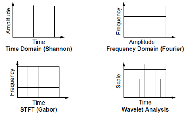
Wavelet analysis allows the use of long time intervals where we want to observe more precise low frequency information, and shorter regions where we want to observe high frequency information. In figure above comparison of FFT, STFT and WT is graphically represented.

Wavelet transform name comes from the fact that it uses a waveform instead of sinusoid function used in Fourier transform. Mother wavelet is waveform of effectively limited duration that has an average value of zero. Wavelet analysis does not use a time-frequency region, but rather a time-scale region. This is because wavelet analysis works by breaking up a signal into shifted and scaled versions of the mother wavelet. Scaling a wavelet means stretching (or compressing) it, where small scale is very compressed signal and large scale is stretched signal. Scale is related to the frequency of the signal in a way that smaller scale means larger frequency and vice versa. Shifting wavelet means delaying it in time. Wavelet transform works in a way that mother wavelet is compared sequentially to sections of the original signal. The result is set of coefficients that are a function of scale and position. These coefficients can be represented and used in many ways. In some cases, inverse transform can be done, which enables to reconstruct signal using only this coefficients.

There are three types of wavelet transform that a commonly used:  continuous wavelet transform (CWT), continuous wavelet transform using FFT (CWTFT) and discrete wavelet transform (DWT). Some of the most important properties of each are listed below.

1.Continuous wavelet transform – CWT

In continuous wavelet transform correlation of signal with mother wavelet can be calculated for any scale and shift of mother wavelet. CWT is calculated in a way that scaled wavelet function is shifted smoothly along the signal and correlation with that signal section is measured.

2. Continuous wavelet transform using FFT – CWTFT

Problem with CWT is that it is redundant and there is no unique way to define inverse. This means that it is not possible to reconstruct signal from coefficients. CWTFT uses FFT of the wavelet function in order to reconstruct signal. Not all wavelet functions can be used in CWTFT. Condition is that it is real value function and that its FFT has support on only positive frequencies. Wavelets that satisfy this admissibility condition are called analytical wavelets.

3. Discrete wavelet transform -DWT

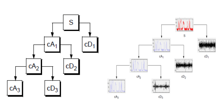
In order to speed up calculation, discrete wavelet transform is used. In DWT “dyadic” (which means based on factor two) scales are used. Even though only few scales are used to cover the whole area of frequencies, transform is much more efficient and equally accurate. In each level of transform signal is decomposed on “detail” and “approximation”. Details are low scale (high frequency) components of signal, while approximations are high scale (low frequency). In each consecutive level approximation is decomposed into detail and new approximation whose scale is smaller and frequency is larger. Iteration of this process results in wavelet decomposition tree. Example of one decomposition tree is shown in figure below. This process could be continued indefinitely in theory, but in practice it is limited with the resolution of the signal. When individual detail consists of a single sample, the end level of decomposition is reached.

Project idea

There is a large repository of papers that were interested in wavelet transform itself and its application on HRV evaluation. It is clear that this is very interesting area and that this technique could further improve understanding of the interactions of the autonomic control systems with the cardiovascular system. In this project idea was to investigate through different approaches which type of wavelet transform is the most appropriate for HRV analysis and what are all the parameters that influence the speed, quality, resolution etc. of the decomposition. Therefore the results of this paper might serve as starting point or component of some future research.

Analysis of wavelet transforms

1.Comparison of methods

Idea was to analyze mentioned three methods of wavelet transform in order to compare them, detect what advantages and drawbacks of each are and to choose the best one on which HRV analysis will be further studied. Several methods were tried; pure coefficients comparison, reconstructed signal comparison, sum of coefficients for each of frequency band of interest (ULF, LF and HF), energy distribution and calculation time comparison.

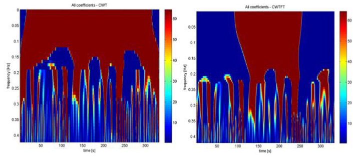
Pure coefficients were compared only for CWT and CWTFT since DWT has only few scale levels. In HF frequency range there is almost no difference between CWT and CWTFT, but as approaching to ULF frequencies differences increase as can be seen in figures below. Unfortunately, appropriate explanation for that was not found but it is believed that it is because of some constraints of CWT for very low frequencies. Also some differences could be caused by slightly different boundary frequencies for frequency bands.

For comparison of reconstructed signals, original signal was reconstructed using coefficients for each frequency band separately. This was only possible to do with CWTFT and DWT method. Again, difference was very small for HF and LF, only for ultra-low frequencies (UFL) difference was more visible, but even then main trends were the same.

In order to compare all three methods at the same time, sum of all coefficients for every frequency band was studied. Results are very similar for all three methods with only minor differences for HF and LF band. For ULF band larger difference for CWT is noticed which agrees with previous results.

Distribution of energy through different frequencies was studied in order to compare methods with Fourier decomposition of signal. The results have shown very good correlation between frequency values of peaks of energy distribution and FFT spectrum.

The last thing to consider was computation time for different methods. CWT method consumes very much time and CPU power. CWTFT takes only few (< 5min) minutes to compute even for signals with almost million samples in comparison to CWT which takes few hours (<3h) for the same task. On the other hand DWT is even faster than CWTFT and it takes under minute to do the decomposition.

Conclusion is that DWT is the best method for the wavelet decomposition for several reasons: time and CPU power consumption, simplicity of decomposition and reconstruction and the quality of decomposition and reconstruction itself.

2.DWT method analysis

1) Quality of decomposition

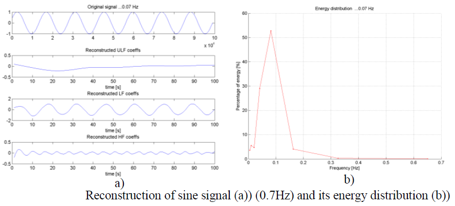
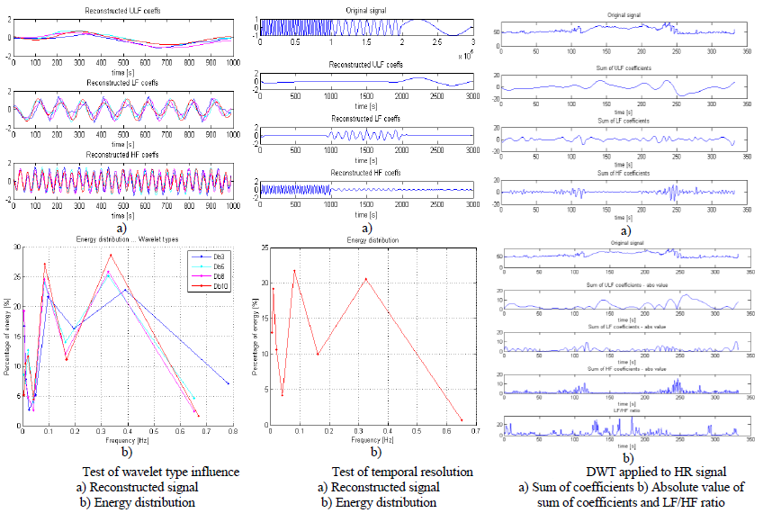
Quality of decomposition was tested using artificial sinusoidal signals of known frequencies. Frequencies within different frequency bands were used. Energy distribution globally and how well the peak of maximal energy corresponds to the frequency of sinusoid was studied. Reconstruction signals using separately HF, LF and ULF frequency bands ware observed (their amplitude and period) too and is shown on figures below. Detection to which band some frequency belongs, based on reconstruction is precisely detected only for frequencies which are in the middle of the frequency band and further from the boundaries. As getting closer to the boundaries other bands detect these frequencies too, but with lower amplitude and wrong period. Also quality of detection based on energy distribution depends whether the frequency is closer or further from one of the frequencies corresponding to the scales that were used in decomposition (since DWT uses dyadic scales). Frequency detection was very precise for ULF and LF band, but less precise for HF band, since for them frequencies resolution is smaller and the error is larger.

2) Noise influence

Signal which consists of sinusoid waves of three different frequencies (each within one frequency band) was used. To this signal two different levels of Gaussian noise were added. Reconstruction and energy distribution for signal with and without noise was studied and is shown on figures below.

Results showed that noise didn’t influence decomposition and reconstruction even when amplitude of noise was in range of signal amplitude. This is another very positive property of DWT transform.

3) Influence of chosen wavelet function

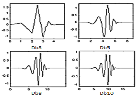
Finally, the influence of chosen mother wavelet function on energy distribution and reconstruction was studied. Four wavelets from Daubechie’s family were used: “db3”, “db5”, “db8” and “db10” as shown in figure below. Result of comparison is that difference is very small for LF and HF band, but for ULF there are noticeable differences. For LF and HF, reconstruction signals look very similar especially for “larger” Daubechie wavelet functions (shown in figure below). It is because larger orders of Daubechie functions are more complex ones, but also more similar to each other than the ones of small order (for example Db1 is actually step function). For this reason for precise calculation it is suggested to use enough large Db wavelet function (>Db8). Last thing to notice is that reconstructed signals in each band are not sinusoid functions as one may expect. This is due to the fact that borders of frequency bands in DWT are not very precise.

4) Temporal resolution

Signal whose frequency content changes in time was used. First part of the signal is sinusoid with frequency of 0.3Hz which is in HF band, then sinusoid of 0.1Hz (LF band) follows and at the end sinusoid of 0.01Hz (ULF band). It can be seen from reconstruction signals for different frequency bands that time detection of each sinusoid within input signal is very precise (shown in figure below). Also energy distribution clearly shows peaks on frequencies values of original signal. This confirms DWT ability to analyze signal in frequency and time domain.

Analysis of HRV using wavelet transform

Five minute signal of heart rate sampled with 500 sample/s is used to present input and output data of HRV analysis using DWT method. In figure above original signal and DWT coefficients separately for ULF; LF and HF frequency band are presented.

As previously mentioned, parasympathetic nervous system (PNS) is major contributor to HF component. Slight disagreement exists in respect to the LF component. Some studies suggest that LF is a quantitative marker of sympathetic (SNS) activity, while other studies view LF as reflecting both sympathetic and parasympathetic activity. Consequently, the LF/HF ratio is sometimes introduced to mirror sympathetic-parasympathetic balance and also to reflect the sympathetic modulations.

LF/HF ratio is obtained by dividing values of LF coefficients with HF coefficients. Absolute value is used because we are interested in “power” of the LF and HF band in time. After division, LF/HF ratio was averaged in time using median filter with a window size of 500 samples which corresponds to one second. This way resolution of LF/HF ration is one second which is reasonable. In order to visually better see connection between LF, HF coefficients and LF/HF ratio in figure above, absolute values of coefficients are plotted.

In this signal HRV during respiration is observed. Such, deep breathing or apnea, tests are usually used in clinical testing or calibrations. During normal uncontrolled breathing respiration seems to influence HRV for less than 10%, but controlled respiration increases this influence up to almost 50% [3.]. During apnea or suspension of breathing, heart rate changes with frequencies in range from 0.01 to 0.04 Hz. This means that power of ULF band of HRV increases. Also at the same time LF/HF ratio is increased [4.] as a consequence of higher sympathetic processes. Similar effect happens during sleep of patients with sleep disordered breathing, where increased LF/HF ratio reflects not only sympathetic dominance but also reduced parasympathetic control [4.]. In the signal on figure above it can be noticed that LF/HF ratio is increased in time between approximately 130th and 230th second. In the same time interval ULF coefficients values are relatively large in comparison to the rest of the time. These two things indicate that at this time interval patient might have suppressed breathing. This could be confirmed if breathing was also recorded at the same time.

Conclusion

In this work, possibility to analyze heart rate variability (HRV) with wavelet transform was investigated. Three methods of wavelet transform were compared (CWT, CWTFT and DWT). Since, DWT showed to be the best one from several reasons: time and CPU power consumption, simplicity of decomposition and reconstruction and in the end quality, it was tested further. Quality of DWT decomposition, noise influence, mother wavelet type influence and time resolution were observed. DWT showed to have high noise robustness, excellent temporal and good frequency resolution, and as such showed to be very good candidate for more precise analyses and someday even usage for other scientific and clinical purposes.

Acknowledgement

This work was done during Erasmus+ exchange on Technical University of Vienna. I would like to thank to my two mentors that gave me opportunity to work on this project and helped me all the way along F.T. and E.K. Short report can be downloaded here: BSS_report

Short student paper about this work was presented on MIPRO conference in Opatija, Croatia in 2016. The paper was published in Proceedings of the 39th International Convention, pp. 1930-1935 and can be downloaded here:  MIPRO_paper

Literature

[1.] E. Kaniusas: Biomedical sensors and signals I, Springer 2012.

[2.] Task Force of the European society of cardiology and the North American society of pacing and electrophysiology: Heart rate variability – Standards of measurement, physiological interpretation, and clinical use, European Heart Journal, 1996

[3.] V. Demchenko,R. Čmejla, J. Vokřál: Analysis of heart rate variability during respiration

[4.] I. Szollosi, H. Krum, D. Kaye, M. T. Naughton: Sleep Apnea in Heart Failure Increases Heart Rate Variability and Sympathetic Dominance, Sleep Journal, 2007.

Typical EMG measurement system consists of one central device with more channels with electrodes which are connected with wires which makes whole system complex and restrictive during movements. Moreover, in general third reference electrode which is placed on electrically non-active tissue further away is used, which limits any smaller and more user friendly designs.

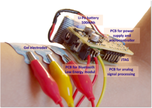
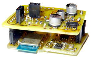
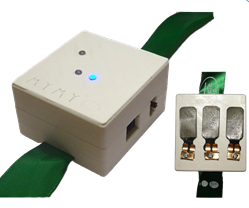
The goal of this project was to design, construct and test a single channel compact-size, wireless and surface EMG measurement system. Idea was that instead of having central device which is used for sampling and processing, each channel is independent acquisition system which can send acquired and processed data wirelessly to a device with graphical user interface. As a wireless communication channel Bluetooth Low Energy used which enabled to have a smart phone as a central device which collects stores and visualizes data. Current maximal transfer data rate achieved with BLE is 770 samples/s. In further work, attempt should be made to achieve 1ksample/s transfer rate.

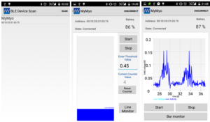
Additionally, three-electrode analog amplification and filtering part was designed, constructed and tested. Final dimensions of device are approx. 4cm x 3cm x 3cm. The device attaches to the body by using three sticky gel electrodes. In Android application the measured data is visualized in two ways: in line graph where data can be observed through time and in bar graph where current muscle activation is visualized.

.                             

In future fatigue analysis part will be added to the Application and logging of the measured data to the SD card. Also more devices will be able to connect simultaneously. Since final idea is to use device for physiotherapy, goal is to be able to define different exercises by muscle activation levels. This way application could analyze exercise performance, count properly done ones and give feedback to the patients.

In total, the prototype of compact-size, wireless and surface EMG measurement device was constructed and tested successfully.

Project was presented on a CMBEBIH  (International Conference on. Medical and Biological Engineering) that was held from 15. to 18. March 2017. in Sarajevo, Bosnia and Herzegovina. A presentation of a project: CMBEBIH_presentation

MyMyo was presented on the 9th “International Exhibition of Inventions” (Kunshan, China) 2016 where it received gold medal  and on 14th “International Innovation Exhibition” (Zagreb, Croatia) 2016 where  it received silver medal. Poster from the exhibitions can be seen here:Exhibitions_poster

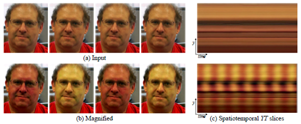
Eulerian video magnification (EVM) is very new technique that enables amplification and thus revealing subtle changes and movements on standard quality videos. It reveals temporal variations in videos that are difficult or impossible to see with naked eye. Since human visual system has limited spatio-temporal sensitivity this could serve as a microscope for videos.

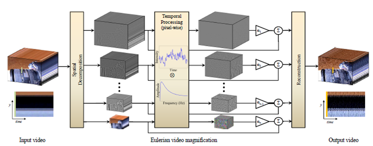
Basic idea and working principle can be seen on picture below [1].

More about it can be found here:

http://people.csail.mit.edu/mrub/vidmag/

https://www.youtube.com/watch?v=ONZcjs1Pjmk

or on this TED https://www.youtube.com/watch?v=fHfhorJnAEI&spfreload=10

Idea of the project

Idea of this project was to evaluate if Eulerian video magnification applied to video recordings of palpation sites of human could be used for contactless heart rate(HR) and pulse transit time (PTT) assessment.

Today still most of the methods to measure heart rate and pulse transit time need contact with skin and some are even invasive. From this reason simple method which is contactless and doesn’t require any special equipment except camera for recording and computer for processing would be of large significance.

EVM principle

In EVM spatio-temporal processing is used to emphasize subtle temporal changes in video. Multiscale analysis is started by computing a full Laplacian pyramid from input video sequence. Levels of Laplacian pyramid can be also called spatial frequency bands. Temporal processing is performed on each spatial band. Values of each pixel in time are observed and a bandpass filter is used to extract the frequency band of interest. The temporal filtering is defined by the type of changes (motion, vibrations etc.) that we want to extract. The same filtering is applied to all spatial levels and to all pixels within each level. Extracted bandpass signal is then multiplied by magnification factor α. In the end magnified signal is added to the original signal and spatial pyramid is collapsed in order to obtain the final output video. All the steps are visually shown on picture below [1].

Measurement setup

Measurement setup consisted of ECG measuring setup, pressure measuring setup, photoplethysmogram (PPG) setup and camera. It was all done at Technical University of Vienna using “Biopac systems” MP36R four-channel data acquisition system. Software used to visualize and log the data was “Biopac Student Lab System” while processing and calculation of recorded signals and video was done using “Matlab”.  These measurements were done simultaneously while video of palpation site was recorded. Video was recorded using “GoPro Here4 Silver” camera using 120 fps and 720×680 px resolution and “normal” field of view. Lightning conditions were good but no extra equipment was used except small table lamp sometimes. The goal was to have simplest and cheapest equipment as possible so that patient could use it eventually at home independently.

Measurement procedure

Measurements were done in a way that first subject was breathing normally for approx. 30 seconds, and then deep breathing was done so that subject could start apnea (breath holding). Apnea lasted approx. 40-60 seconds, and after it subject was recorded for next approx. 20 seconds.

This procedure was chosen because during it blood pressure changes significantly. At the beginning pressure is at some normal value for the resting condition. During breath holding pressure starts to drop and reaches minimal value, and then starts to rise and reaches maximal value. This way at least three different time and pressure ranges can be chosen in order to compare PTT calculated from video and EVM and measured pressure.

Different palpation sites were used in order to compare results and find the best palpation sites for HR measurement and best pair of palpation sites for blood pressure assessment. On following pictures frames from videos where different palpation pairs were used are shown. Even between two wrists or two toes there should be PTT difference because heart is moved a little to the left side of the chest.

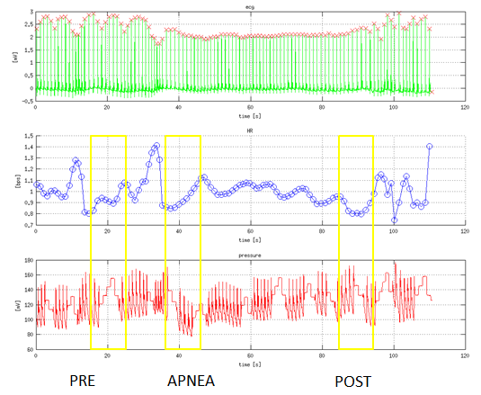
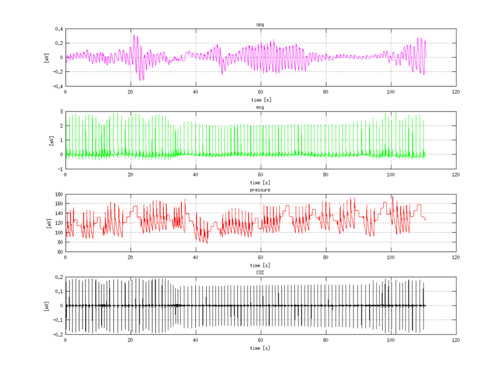
Example of recorded signals is shown on next picture. First signal is photoplethysmogram (PPG), then electrocardiogram (ECG) and third measured is pressure. Fourth signal is CO2 consumption which was not measured but computed, and is not important for the project.

HR assesment

There are several sites on the body where a pulse can be measured. All arteries have a pulse, but it is easier to palpate the pulse at locations where artery is near the surface of the skin and when there is firm tissue (such as a bone) beneath the artery. The three most common sites are the radial (wrist), carotid (throat), and brachial (inside of elbow).

Basic steps in order to extract heart rate from bare video are:

1. selection region of interest (ROI) in order to reduce computational efforts and reduce error probabilities
2. computing EVM of the ROI
3. calculating average FFT of amplified ROI

Calculating average FFT was not as easy as it seems. There was a question if it is better to calculate average FFT or FFT of average. Average FFT showed to be more reliable and robust.

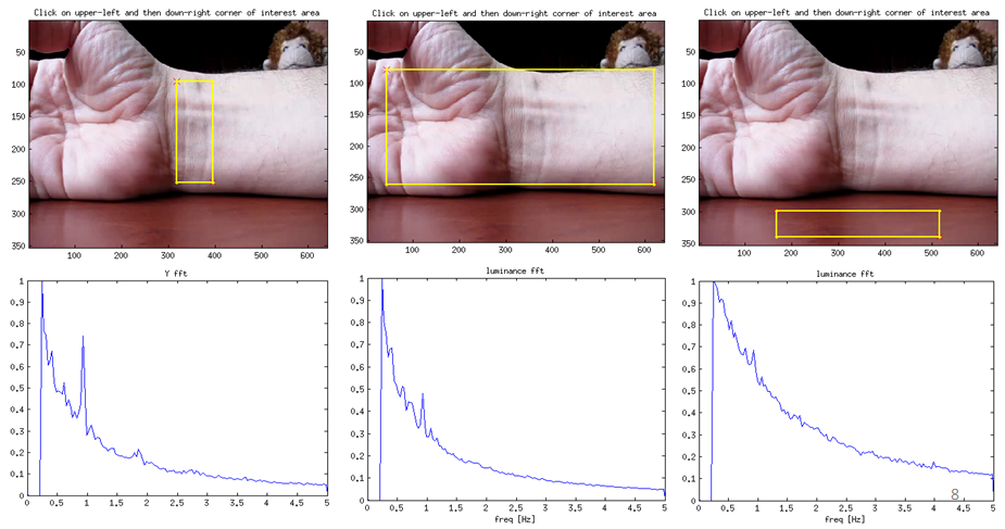
The second thing that needed testing was which pixels of ROI are actually the interesting ones. This happens because the ROI is usually general area around palpation site, not really area of vessel with amplified movements, because it’s hard and unrealistic to expect that person can select exactly place with larger vessel movements. There were few things tried:  using all pixels in ROI, using only middle line and using only pixels with largest amplitude values

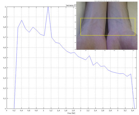
On the image below dependence of HR assessment depending on the ROI selection is shown. 

In order to really compare HR calculated using EVM method from video and real HR measured with ECG, HR was calculated from ECG. HR was calculated in “Matlab” using function that recognizes QRS peaks. When peaks were recognizes program calculates time interval between two neighboring peaks 𝑇𝑝𝑝 and calculates heart rate 𝑓ℎ𝑟 as 1/𝑇𝑝𝑝 for each two neighboring QRS peaks. Example of HR (𝑓ℎ𝑟) calculated and plotted in time is on picture below.

On real HR signal time range (10s) with relatively constant HR was selected (as shown on picture above). Video cut-out of 10s with time stamps where HR was constant was used only. ROI was selected and amplified, pixel values in time evaluated and FFT from this 10s cut-out was calculated. If video was shorter it would be easier to find constant HR value, but resolution of FFT would not enable to precisely determine frequency of real peak. This way 10s time was compromise between resolution and precision of FFT calculation and possibility to find HR region with relatively constant value.

The calculated HR (corresponding FFT) is shown on a figure below. It can be seen that HR is determined precisely. This was tested and confirmed on more moments (cut outs) of HR signal.

Pulse transit time assessment

The velocity at which the arterial pulse propagates is called the “pulse wave velocity” (PWV). PWV is used as a measure of arterial stiffness. It is easy to measure it invasively and non-invasively in humans and is highly reproducible. It’s important because it has a strong correlation with cardiovascular events and all-cause mortality.

The equation that directly relates PWV and artery wall stiffness is called Moens-Korteweg equation. PWV increases with pressure because arterial compliance decreases with increasing pressure (due to curvilinear relationship between arterial pressure and volume). Volume increases with increasing pressure because artery dilates which directly increases PWV. PWV approximately increases with a rate of 1m/s per 100mmHg pressure.

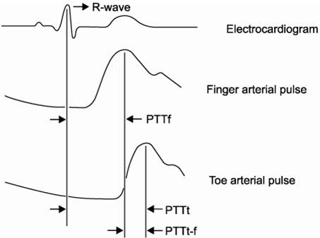
Pulse transit time is generally time difference of pulse wave signal coming to two different places in body. If the first place is heart than it can also be called PAT. In picture below PTT between three different places are shown; PTTf – PTT from heart to finger, PTTt – PTT from heart to toe and PTTt-f – PTT from finger to toe.

Since PTT is directly connected to pulse wave velocity (PWV) it is suitable as an indirect measure of blood pressure change. Exactly this fact will be used to evaluate if this method works, and if it can be used to measure blood pressure. Of course that calibration would be needed at the beginning, since PWV and PTT are related to pressure change and not to absolute value of pressure.

Idea was to record two palpation places at the same time with one camera, extract pulse signals on both of them and measure time shift between them. Time shift is related to PWV and PWV is related to blood pressure.

First, person selects two regions of interest (ROIs). First selected (ROI1) is the one that is further from the heart and the second one is the one closer to the heart (ROI2). Two videos are made, one for each ROI because in case of making EVM with original video computation was time and memory restricted. Newly composed videos are loaded and each is amplified separately but with same EVM parameters.

Average signal in time was calculated for both of the videos. Next step was filtering these time signals with frequency range of interest. Instead of first-order IIR filter suggested in [1] for motion amplification ideal bandpass filter was used. The problem with IIR filter was that borders were too broad and actually it was not clear which frequencies are contained in the filtered signal and which are not, and that made further calculation worse. Frequency band that was most often used was [0.75, 1.25]Hz, but in future the idea is to find HR with FFT as previously described and then filter with range [HR-25%HR,HR+25%HR]. This 25% width could be altered depending on the quality of results.

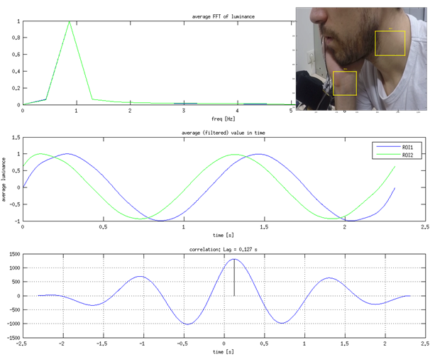
The last step is to calculate time shift between time signals of two ROIs. This is done calculating correlation between two signals. PTT is time value where correlation is maximal. PTT has to be positive, because of agreement which one is ROI1 and which ROI2 during selection.

An example of video frame with two ROI selection, FFTs and average signals in time for both ROIs and calculated correlation are shown on figure below.

There is still lot of work with PTT assessment and relating it to blood pressure, but preliminary experiments were done. First experiment was to measure PTT for different pairs of palpation places. For each pair average PTT for ~10 measurements was done and approximated difference of distances of palpation places from heart was measured. Measurements were different selections of ROIs on the same video. Idea was to compare calculated PWV for all palpation pairs. First results are shown in table below.

Even though approx. PWV are not the same, they are relatively similar and fit into the frame of possible PWV values for young person. More experiments and more thorough evaluation are needed. Plan is to test with even more different selections of ROIs, to make different videos of the same subject and also to use more different subjects.

 Blood pressure assessment

Absolute value of PTT or calculated value of PWV doesn’t tell much actually, because it depends on many individual parameters for each person. Also most of these parameters are not even easily measurable. PTT and PWV are related with blood pressure, but PWV and PTT could not be used to determine absolute value of blood pressure, but to detect changes in pressure, which is also very useful indicator. Since only change in pressure could be determined, calibration would be needed for each patient in order to know some starting pressure values.

In order to test if there is correct correlation between PTT (and PWT) measured with EVM method and real pressure differences a measurement with voluntary apnea is used. Measurement was processed in a way that from pressure recording three regions were selected; before apnea where pressure was of an average value, during apnea where pressure reached minimal value and after apnea at the moment when pressure reached maximal value as shown in picture below. Each region was 5 seconds long so that videos would be enough long to precisely determine correlation between signals. Idea was to plot PTT vs pressure.

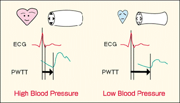
If blood pressure is high, arterial walls are tenser and more firm which causes the pulse wave to travel faster. This means that PWV is larger and PTT is shorter. From this follow some basic expectations as written in table below. Simple illustration is also shown on a picture below.

Current measurements were done using different palpation pairs from one video of only one person. At the moment calculated PTT from measurements doesn’t follow the expectations from table above. PTT times are way too large, meaning that PWV calculated from them are not possible. There are few suspicions why this happened. One of them is that video recordings were not good, because even when amplified, motion is barely visible (which is not typical after amplification). Possible is that regions were not zoomed enough, that lightning conditions were not enough good, and that hand or neck were not enough still during recording and that maybe some holders should be used. It is possible that movement of hand or neck is extracted and analyzed instead of vessel vibration. More probable is that parameters of EVM amplification were not good enough. In EVM amplification algorithm parameters are amplification, spatial wavelength, frequency borders and levels of Laplacian pyramid. It was assumed that those parameters can be the same for all videos and all palpation pairs but maybe this is not true. All these things need to be further investigated.

Acknowledgement

This project was done during semester at Erasmus exchange at Technical University of Vienna. Many thanks goes to mentors  F.T. and E.K. without whose support this wouldn’t be done.

Literature

[1.] H. Wu, M. Rubinstein, E. Shih, J. Guttag, F. Durand, W. Freeman: Eulerian Video Magnification for Revealing Subtle Changes in the World
[2.] Jeong, I. Cheol, J. Finkelstein: Introducing Contactless Blood Pressure Assessment Using a High Speed Video Camera
[3.] EJ. Kim, CG. Park, JS. Park, SY. Suh, CU. Choi, JW. Kim, SH. Kim, HE. Lim, SW. Rha, HS. Seo, DJ. Oh: Relationship between blood pressure parameters and pulse wave velocity in normotensive and hypertensive subjects: invasive study
[4.] E. Kaniusas: Biomedical sensors and signals I, Springer 2012.
[5.] P. Boloto Chambino: Android-based implementation of Eulerian Video Magnification for vital signs monitoring
[6.] M. Estrada, A. Stowers: Amplification of Heart Rate in Multi-Subject Videos
[7.] M.A.Elgharib, M. Hefeeda, F. Durand, W.T.Freeman: Video Magnification in Presence of Large Motions